Excel VBAで条件付き書式をクリアし設定する方法:セル Tips
条件付き書式をVBAで使うのは割と簡単で、FormatConditionsで全て行います。
クリアはDelete、設定はAdd、書式設定はFormatConditionsの引数で行います。
FormatConditions.Addの構文
FormatConditions.Add( Type, Operator, Formula1, Formula2 )
- Type : (省略不可)セル値または演算式のどちらを基に条件付き書式を設定するかを指定
- Operator : (省略可)条件付き書式の演算子を指定
- Formula1 : (省略可)条件付き書式に関連させる値またはオブジェクト式を指定
- Formula2 : (省略可)OperatorにxlBetweenかxlNotBetweenを指定した場合、条件付き書式の 2 番目の部分に関連させる値またはオブジェクト式を指定
| 名前 | 値 | 内容 |
| xlCellValue | 1 | セルの値 |
| xlExpression | 2 | 演算 |
| xlColorScale | 3 | カラースケール |
| xlDatabar | 4 | データバー |
| xlTop10 | 5 | トップ10 |
| XlIconSet | 6 | アイコン セット |
| xlUniqueValues | 8 | 一意の値 |
| xlTextString | 9 | xlTextString |
| xlBlanksCondition | 10 | 空白の条件 |
| xlTimePeriod | 11 | 期間 |
| xlAboveAverageCondition | 12 | 平均以上の条件 |
| xlNoBlanksCondition | 13 | 空白の条件なし |
| xlErrorsCondition | 16 | エラー条件 |
| xlNoErrorsCondition | 17 | エラー条件なし |
Operatorの設定値
| 名前 | 値 | 内容 |
| xlBetween | 1 | 次の値の間 |
| xlNotBetween | 2 | 次の値の間以外 |
| xlEqual | 3 | 次の値に等しい |
| xlNotEqual | 4 | 次の値に等しくない |
| xlGreater | 5 | 次の値より大きい |
| xlLess | 6 | 次の値より小さい |
| xlGreaterEqual | 7 | 次の値以上 |
| xlLessEqual | 8 | 次の値以下 |
ここでは下記のことを掲載しています。
- 指定値と一致すればセルの文字色と背景色を変更する
- 上と同じ処理をFor NextとIF文で行う
- 指定した範囲の値と一致すればセルの文字色と背景色を変更する
- 複数の条件付き書式を設定する
Homeに戻る > Excel セルのTipsへ
下の販売表に条件付き書式を設定します。
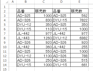
セルの値が1000ならば背景色をRGB(220, 220, 220)に、フォント色を赤にします。
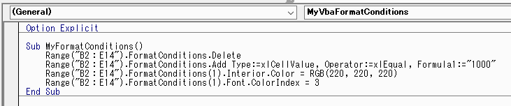
Range("B2:E14").FormatConditions.Delete
Range("B2:E14").FormatConditions.Add Type:=xlCellValue, Operator:=xlEqual, Formula1:="1000"
Range("B2:E14").FormatConditions(1).Interior.Color = RGB(220, 220, 220)
Range("B2:E14").FormatConditions(1).Font.ColorIndex = 3
End Sub
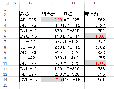
実行結果です。
1000のセルの背景色とフォント色が変更されています。
上と同じ処理をFor NextとIF文のVBAにしてみました。
条件付き書式のFormatConditionsを使った方が、簡単で分かり易そうです。
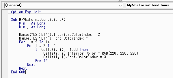
Sub MyVbaFormatConditions()
Dim i As Long
Dim j As Long
Range("B2:E14").Interior.ColorIndex = 2
Range("B2:E14").Font.ColorIndex = 1
For i = 2 To 14
For j = 2 To 5
If Cells(i, j) = 1000 Then
Cells(i, j).Interior.Color = RGB(220, 220, 220)
Cells(i, j).Font.ColorIndex = 3
End If
Next
Next
End Sub
Range("B2:E14").FormatConditions.Delete
Range("B2:E14").FormatConditions.Add Type:=xlCellValue, Operator:=xlBetween, Formula1:="300", Formula2:="600"
Range("B2:E14").FormatConditions(1).Interior.Color = RGB(220, 220, 220)
Range("B2:E14").FormatConditions(1).Font.ColorIndex = 3
End Sub
範囲を設定した実行結果です。
Range("B2:E14").FormatConditions.Delete
Range("B2:E14").FormatConditions.Add Type:=xlCellValue, Operator:=xlBetween, Formula1:="300", Formula2:="600"
Range("B2:E14").FormatConditions(1).Interior.Color = RGB(220, 220, 220)
Range("B2:E14").FormatConditions(1).Font.ColorIndex = 3
Range("B2:E14").FormatConditions.Add Type:=xlCellValue, Operator:=xlEqual, Formula1:="1000"
Range("B2:E14").FormatConditions(2).Font.ColorIndex = 4
Range("B2:E14").FormatConditions.Add Type:=xlCellValue, Operator:=xlEqual, Formula1:="977"
Range("B2:E14").FormatConditions(3).Font.ColorIndex = 5
End Sub
実行結果です。
指定値と一致すればセルの文字色と背景色を変更する
条件付き書式のVBAです。セルの値が1000ならば背景色をRGB(220, 220, 220)に、フォント色を赤にします。
- FormatConditions.Delete : 設定済みの条件付き書式をクリアします。
- Add : 条件付き書式を設定します。
- Type:=xlCellValue : セルの値が
- Operator:=xlEqual : 次の値に等しい場合
- Formula1:="1000" : 値に1000をセット
- Interior.Color : セルの背景色
- Font.ColorIndex : フォント色
Range("B2:E14").FormatConditions.Delete
Range("B2:E14").FormatConditions.Add Type:=xlCellValue, Operator:=xlEqual, Formula1:="1000"
Range("B2:E14").FormatConditions(1).Interior.Color = RGB(220, 220, 220)
Range("B2:E14").FormatConditions(1).Font.ColorIndex = 3
End Sub
実行結果です。
1000のセルの背景色とフォント色が変更されています。
上と同じ処理をFor NextとIF文のVBAにしてみました。
条件付き書式のFormatConditionsを使った方が、簡単で分かり易そうです。
Sub MyVbaFormatConditions()
Dim i As Long
Dim j As Long
Range("B2:E14").Interior.ColorIndex = 2
Range("B2:E14").Font.ColorIndex = 1
For i = 2 To 14
For j = 2 To 5
If Cells(i, j) = 1000 Then
Cells(i, j).Interior.Color = RGB(220, 220, 220)
Cells(i, j).Font.ColorIndex = 3
End If
Next
Next
End Sub
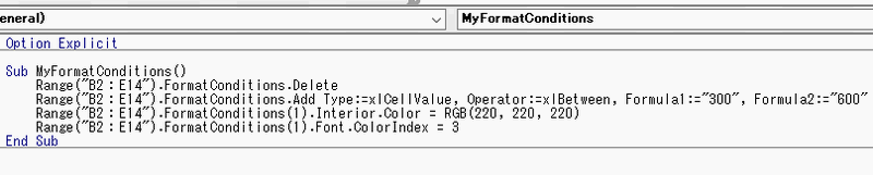
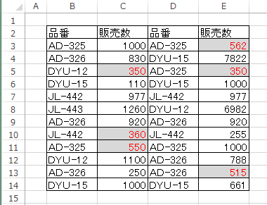
指定した範囲の値と一致すればセルの文字色と背景色を変更する
セルの値が300から600の範囲ならば背景色と文字色を変更します。- OperatorをxlBetweenにし、Formula1とFormula2を設定しています。
- FormatConditions(1)に、背景色と文字色の書式を設定しています。
Range("B2:E14").FormatConditions.Delete
Range("B2:E14").FormatConditions.Add Type:=xlCellValue, Operator:=xlBetween, Formula1:="300", Formula2:="600"
Range("B2:E14").FormatConditions(1).Interior.Color = RGB(220, 220, 220)
Range("B2:E14").FormatConditions(1).Font.ColorIndex = 3
End Sub
範囲を設定した実行結果です。
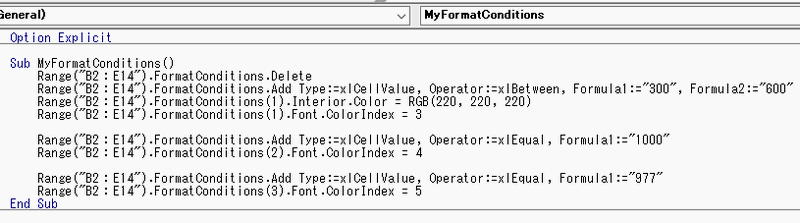
複数の条件付き書式を設定する
300から600の範囲設定、1000の場合、977の場合の3つの条件付き書式を設定しています。- 1つ目の300から600の範囲設定は、FormatConditions(1)で行います。
- 2つ目の1000の場合は、FormatConditions(2)で行います。
- 3つ目の977の場合は、FormatConditions(3)で行います。
Range("B2:E14").FormatConditions.Delete
Range("B2:E14").FormatConditions.Add Type:=xlCellValue, Operator:=xlBetween, Formula1:="300", Formula2:="600"
Range("B2:E14").FormatConditions(1).Interior.Color = RGB(220, 220, 220)
Range("B2:E14").FormatConditions(1).Font.ColorIndex = 3
Range("B2:E14").FormatConditions.Add Type:=xlCellValue, Operator:=xlEqual, Formula1:="1000"
Range("B2:E14").FormatConditions(2).Font.ColorIndex = 4
Range("B2:E14").FormatConditions.Add Type:=xlCellValue, Operator:=xlEqual, Formula1:="977"
Range("B2:E14").FormatConditions(3).Font.ColorIndex = 5
End Sub
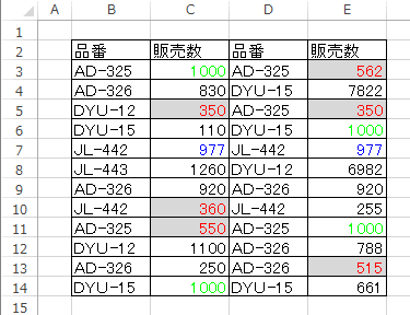
実行結果です。
- セルの値が300から600の背景色が、灰色で文字が赤色で表示されています。
- セルの値が1000の場合、緑色で表示されています。
- セルの値が977の場合、青色で表示されています。
Homeに戻る > Excel セルのTipsへ
■■■
このサイトの内容を利用して発生した、いかなる問題にも一切責任は負いませんのでご了承下さい
■■■
当ホームページに掲載されているあらゆる内容の無許可転載・転用を禁止します
Copyright (c) Excel-Excel ! All rights reserved